Logistic Growth

In logistic growth, a population’s per capita growth rate gets smaller and smaller as population size approaches a maximum imposed by limited resources in the environment.

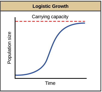
Exponential growth may happen for a while, if there are few individuals and many resources. But when there number of individuals gets large enough, resources start to get used up, slowing the growth rate. Eventually, the growth rate will plateau, or level off, making an S-shaped curve. The population size at which it levels off, which represents the maximum population size a particular environment can support, is called the carrying capacity, or $K$.

Logistic growth can be modeled by modifying the equation for exponential growth, using an $r$ (per capita growth rate) that depends on population size ($N$) and how close it is to carrying capacity ($K$). Assuming that the population has a base growth rate of $r_{max}$ when it is very small, we can write the following equation:

$dN/dT=r_{max}\frac{K-N}{K}N$

At any given point in time during a population’s growth, the expression $K-N$ tells us how many more individuals can be added to the population before it hits carrying capacity. $(K-N)K$, then, is the fraction of the carrying capacity that has not yet been “used up.” The more carrying capacity that has been used up, the more the $(K-N)/K$ term will reduce the growth rate.

When the population is tiny $N$ is very small compared to $K$. The $(K-N)/K$ term becomes approximately $(K/K)$, or 1, giving us back the exponential equation. This fits with our graph above: the population grows near-exponentially at first, but levels off more as it approaches $K$.

Examples of Logistic Growth

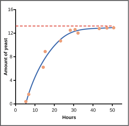
Yeast, a microscopic fungus used to make bread and alcoholic beverages, can produce a classic S-shaped curve when grown in a test tube. In the graph shown below, yeast growth levels off as the population hits the limit of the available nutrients. (If we follow the population for longer, it would likely crash, since the test tube is as closed system – meaning that fuel sources would eventually run out and wastes might reach toxic levels).

In the real world, there are variation of the “ideal” logistic curve. For example in the growth below, which illustrates population growth in harbor seals in Washington State. In the early part of the 20th century, seals were actively hunted under a government program that viewed them as harmful predators, greatly reducing their numbers. Since the program was shut down, seal populations have rebounded in a roughly logistic pattern.

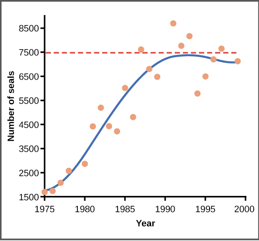
As shown in the graph above, population size may bounce around a bit when it gets to carrying capacity, dipping below or jumping above this value. It’s common for real populations to oscillate (bounce back and forth) continually around carrying capacity, rather than forming a perfectly flat line.