Exponential & Logistic Growth

Key Points

• In exponential growth, a population’s per capita (per individual) growth rate stays the same regardless of population size, making the population grow faster and faster as it gets larger.
• In nature, populations may grow exponentially for some period, but they will ultimately be limited be resource availability.
• In logistic growth, a population’s per capita growth rate gets smaller and smaller as population size approaches a maximum imposed by limited resources in the environment, known as the carrying capacity (K)
• Exponential growth produced a J-shaped curve, while logistic growth produces an S-shaped curve.

Introduction

In theory, any kind of organism could take over the Earth by just reproducing. For instance, imagine a single pair of male and female rabbits. If these rabbits and their descendants reproduced at top speed for 7 years, without any deaths, there would have enough rabbits to cover the entire state of Rhode Island. In another example, a single bacterium of E. coli could cover the Earth with a 1-foot layer in just 36 hours. However, all living organisms need specific resources, such as nutrients and suitable environments, to survive and reproduce. These resources aren’t unlimited, and a population can only reach a size that matches the availability of resources in its local environment.

Population ecologists use a variety of mathematical methods to model population dynamics (how populations change in size and composition over time). Some of these models represent growth without environmental constraints, while others include “ceilings” determined by limited resources. Mathematical models of populations can be used to accurately describe changes occurring in a population and, importantly, predict future changes.

Modeling Population Growth Rates

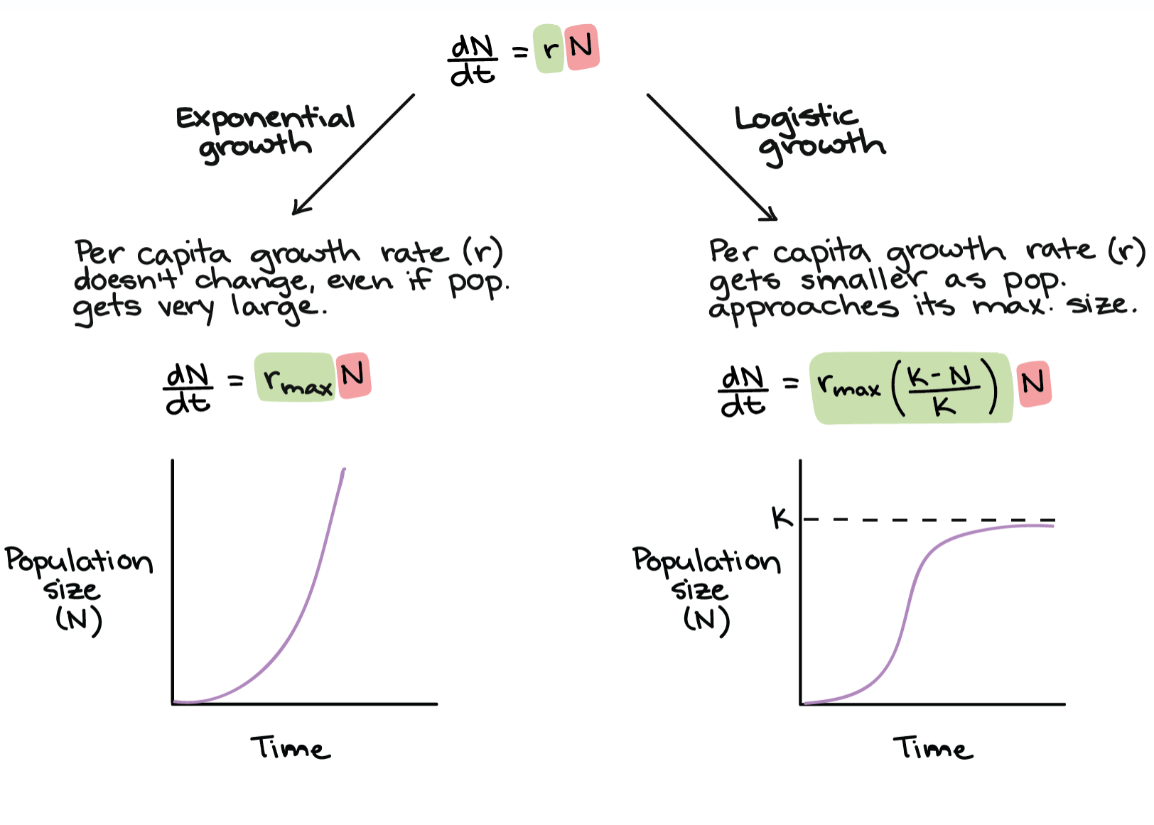
The general equation for population growth rate (change in number of individuals in a population over time) is:

$\frac{dN}{dT}=rN$

In this equation, $dN/dT$ is the growth rate of the population in a given instant, $N$ is population size, $T$ is time, and $r$ is the per capita rate of increase –that is, how quickly the population grows per individual already in the population.

If we assume no movement into or out of the population, $r$ is just a function of birth and death rates.

The equation above is very general, and there are more specific forms of it to describe two different kinds of growth models: exponential and logistic.

• When the per capita rate of increase ($r$) takes the same positive value regardless of the population size, then it becomes exponential growth.
• When the per capita rate of increase ($r$) decreases as the population increases towards a maximum limit, then it becomes logistic growth.

The following is a preview of the growth models.

Exponential Growth

In exponential growth, the population’s growth rate increases over time, in proportion to the size of the population. As an example for exponential growth, we will use bacteria grown in labs.

Bacteria reproduce by binary fission (splitting in half), and the time between divisions is about an hour for many bacterial species. To see this exponential growth, let’s start by placing 1000 bacteria in a flask with an unlimited supply of nutrients.

• After 1 hour, each bacterium will divide, yielding 2000 bacteria (an increase of 1000$bacteria).
• After 2 hours, each of the 2000 bacteria will divide, producing 4000 (an increase of 2000 bacteria).
• After 3 hours, each of the 4000 bacteria will divide, producing 8000 (an increase of 4000 bacteria).

The key concept of exponential growth is that the population growth rate—the number of organisms added in each generation—increases as the population gets larger. And the result can be dramatic: after 1 day (24 cycles of division), our bacterial population would have grown from 1000 to over 16 billion. When population size, $N$, is plotted over time, a J-shaped growth curve is made.

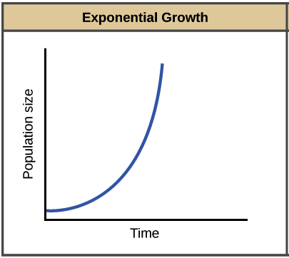
The result is an exponential growth when $r$ (the per capita rate of increase) for the population is positive and constant. While any positive, constant $r$ can lead to an exponential growth, you will often see exponential growth represented with an $r$ of $r_{max}$.

$r_{max}$ is the maximum per capita rate of increase for a particular species under ideal conditions, and it varies from species to species. For instance, bacteria can reproduce much faster than humans, and would have a higher maximum per capita rate of increase. The maximum population growth rate for a species, sometimes called its biotic potential, is expressed in the following equation:

$\frac{dN}{dT}=r_{max}N$

Logistic Growth

Exponential growth is not a very sustainable state of affairs, since it depends on infinite amounts of resources (which tend not to exist in the real world). Logistic growth is a more accurate representation of population size.

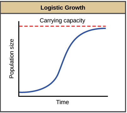
Exponential growth may happen for a while, if there are few individuals and many resources. But when there number of individuals gets large enough, resources start to get used up, slowing the growth rate. Eventually, the growth rate will plateau, or level off, making an S-shaped curve. The population size at which it levels off, which represents the maximum population size a particular environment can support, is called the carrying capacity, or $K$.

Logistic growth can be modeled by modifying the equation for exponential growth, using an $r$ (per capita growth rate) that depends on population size ($N$) and how close it is to carrying capacity ($K$). Assuming that the population has a base growth rate of $r_{max}$ when it is very small, we can write the following equation:

$\frac{dN}{dT}=r_{max}\frac{K-N}{K}N$

At any given point in time during a population’s growth, the expression $K-N$ tells us how many more individuals can be added to the population before it hits carrying capacity. $(K-N)K$, then, is the fraction of the carrying capacity that has not yet been “used up.” The more carrying capacity that has been used up, the more the $(K-N)/K$ term will reduce the growth rate.

When the population is tiny $N$ is very small compared to $K$. The $(K-N)/K$ term becomes approximately $(K/K)$, or 1, giving us back the exponential equation. This fits with our graph above: the population grows near-exponentially at first, but levels off more as it approaches $K$.

What factors determine carrying capacity?

Basically, any kind of resource important to a species’ survival can act on a limit. For plants, the water, sunlight, nutrients, and the space to grow are some key resources. For animals, important resources include food, water, shelter, and nesting space. Limited quantities of these resources result in competition between members of the same population, or intraspecific competition (intra- = within; -specific = species).

Intraspecific competition for resources may not affect populations that are well below their carrying capacity—resources are plentiful and all individuals can obtain what they need. However, as population size increases, the competition intensifies. In addition, the accumulation of waste products can reduce an environment’s carrying capacity.

Examples of Logistic Growth

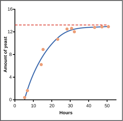
Yeast, a microscopic fungus used to make bread and alcoholic beverages, can produce a classic S-shaped curve when grown in a test tube. In the graph shown below, yeast growth levels off as the population hits the limit of the available nutrients. (If we follow the population for longer, it would likely crash, since the test tube is as closed system – meaning that fuel sources would eventually run out and wastes might reach toxic levels).

In the real world, there are variation of the “ideal” logistic curve. For example in the growth below, which illustrates population growth in harbor seals in Washington State. In the early part of the 20th century, seals were actively hunted under a government program that viewed them as harmful predators, greatly reducing their numbers. Since the program was shut down, seal populations have rebounded in a roughly logistic pattern.

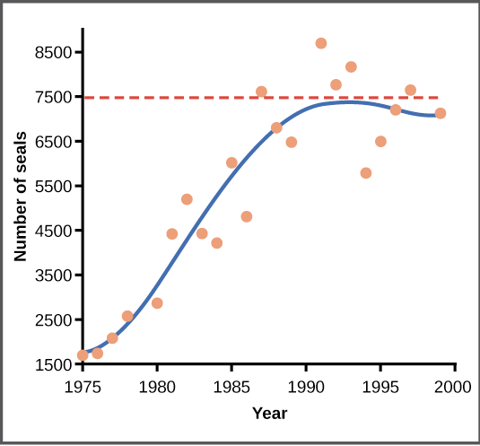
As shown in the graph above, population size may bounce around a bit when it gets to carrying capacity, dipping below or jumping above this value. It’s common for real populations to oscillate (bounce back and forth) continually around carrying capacity, rather than forming a perfectly flat line.